Element Definition

Accelerator elements in LAURA are based on a hierarchical structure. All elements must define some common properties in order to identify their type, machine_area, and other fields. From this base level, additional details can be added progressively depending on the element type and its intended use.

These generic classes are outlined below; refer to Fig. 1 for an inheritance diagram.

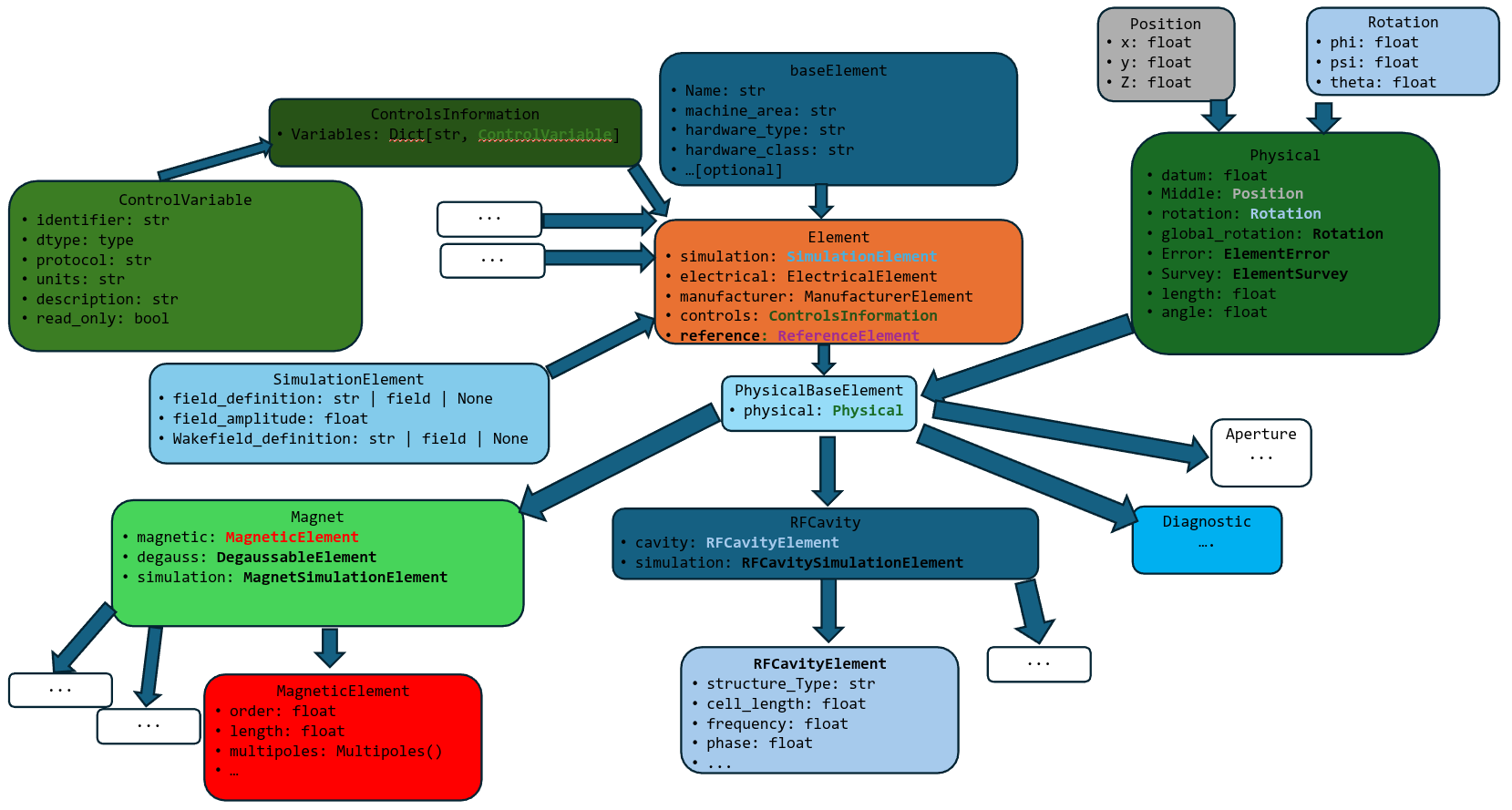
../_images/element-structure.png — Fig. 1 Class structure of `LAURA` elements.

Base-level element

All elements in a LAURA lattice derive from the baseElement class. At a minimum, each element must define:

name: str: The (unique) name of the element.
hardware_class: str: The generic type of the element.
hardware_type: str: The element type. For example, a Quadrupole has hardware_type='Quadrupole' and hardware_class='Magnet'.
machine_area: str: Used for dividing the lattice into sections based on position.

The following additional properties can also be provided:

hardware_model: str: A specific model type of an element, for example the manufacturer name.
virtual_name: str: The name of the element in the virtual control system (if it exists).
alias: str | list: Alternative name(s) for the element.
subelement: bool: Represents whether the element ‘belongs’ to another, i.e. if they overlap in physical space, such as a wakefield attached to a cavity or a solenoid magnet around an RF photoinjector.

While most elements that are typically considered part of an accelerator lattice are defined with reference to a fiducial position, and therefore are described in physical space with respect to that position, not all elements supported by the LAURA standard need to have their position defined. Objects that control lighting, low-level RF modules, RF modulators, or feedback systems, are all examples of elements that derive from baseElement but do not have a physical position defined.

Example: Creating a basic element without physical position:

from laura.models.element import baseElement

# RF modulator - no physical position needed
modulator = baseElement(
    name="MOD-KLYS-01",
    hardware_class="RF",
    hardware_type="Modulator",
    hardware_model="ScandiNova-K100",
    machine_area="KLYSTRON_GALLERY",
    virtual_name="MOD:KLYS:01",
    alias=["mod1", "klystron_mod_1"]
)

# BPM embedded in a quadrupole (subelement)
embedded_bpm = baseElement(
    name="BPM-QUAD-01",
    hardware_class="Diagnostic",
    hardware_type="BPM",
    machine_area="LINAC-1",
    subelement=True
)

Physical element

The PhysicalBaseElement class derives from baseElement, with the additional physical property based on the PhysicalElement class. This allows the position and rotation of the element in Cartesian co-ordinates to be defined. Furthermore, elements can be specified with error and survey attributes, both of which define a position and rotation.

The full specification of an element position therefore consists of:

position: Position(x, y, z) – this refers to the middle of the element.
global_rotation: Rotation(phi, psi, theta)
length: float
angle: float – this is a simplified way of retrieving the bend angle in the X-Z plane.
error: ElementError(position=Position(x, y, z), rotation=Rotation(phi, psi, theta)) – see ElementError; the reference position for an error is the middle of the element.
survey: ElementSurvey(position=Position(x, y, z), rotation=Rotation(phi, psi, theta)) – see ElementSurvey.

Example: Creating elements with physical properties:

from laura.models.element import PhysicalBaseElement
from laura.models.physical import PhysicalElement, Position, Rotation, ElementError

# Quadrupole with position and alignment error
quad = PhysicalBaseElement(
    name="QUAD-02",
    hardware_class="Magnet",
    hardware_type="Quadrupole",
    machine_area="LINAC-1",
    physical=PhysicalElement(
        length=0.5,
        middle=Position(x=0, y=0, z=10.0),
        error=ElementError(
            position=Position(x=0.0001, y=-0.0002, z=0),  # 0.1mm X, -0.2mm Y offset
            rotation=Rotation(phi=0, psi=0, theta=0.001)  # 1 mrad roll
        )
    )
)

# Access computed positions
print(f"Quad start: {quad.physical.start.z}")  # 9.75
print(f"Quad end: {quad.physical.end.z}")      # 10.25

Element

On top of the PhysicalBaseElement, additional information pertaining to a given element can be specified in the Element class, which defines the following additional properties (described in more detail in Auxiliary Classes):

simulation: SimulationElement – see Simulation Element.
controls: ControlsInformation – see Controls Information.
manufacturer: ManufacturerElement – see Electrical, Manufacturer and Reference Information.
electrical: ElectricalElement – see Electrical, Manufacturer and Reference Information.

Example: Complete element definition with all properties:

from laura.models.element import Quadrupole
from laura.models.magnetic import Quadrupole_Magnet
from laura.models.simulation import MagnetSimulationElement
from laura.models.control import ControlsInformation, ControlVariable

# Full quadrupole definition
quad = Quadrupole(
    name="QUAD-MATCH-01",
    machine_area="MATCHING",
    physical={
        "length": 0.3,
        "middle": [0, 0, 15.0],
    },
    magnetic=Quadrupole_Magnet(
        k1l=5.2,  # Normalized gradient
        length=0.31 # Magnetic length
    ),
    electrical={
        "maxI": 250.0,
        "minI": 0.0,
        "read_tolerance": 0.01
    },
    manufacturer={
        "manufacturer": "Sigma Phi",
        "model": "QF-250",
        "serial_number": "2023-001"
    },
    simulation=MagnetSimulationElement(
        n_kicks=10,
    ),
    controls=ControlsInformation(
        variables={
            "READ": ControlVariable(
                identifier="QUAD:MATCH:01:BACT",
                dtype=float,
                protocol="CA", # EPICS channel access
                units="A",
                description="Quadrupole read current",
                read_only=True
            )
        }
    )
)

# Direct attribute access across nested models
print(quad.k1l)            # 5.2 (finds magnetic.k1)

For more examples of creating elements and combining them into lattices, see Examples. Elements can be organized into Section Lattice and Machine Layout structures as described in Lattice Definition. Once defined, elements can be exported to simulation codes using the Translator Module module.

Alternative: Element definition using dictionaries:

from laura.models.element import Quadrupole

# Same quadrupole using dictionary notation
# LAURA automatically converts dictionaries to appropriate class instances
from laura.models.element import Quadrupole

# Same quadrupole using dictionary notation
# LAURA automatically converts dictionaries to appropriate class instances
quad = Quadrupole(
    name="QUAD-MATCH-01",
    machine_area="MATCHING",
    physical={
        "length": 0.3,
        "middle": [0, 0, 15.0],
        "error": {
            "position": [0.0001, -0.0002, 0],
            "rotation": [0, 0, 0.001],
        }
    },
    magnetic={
        "k1l": 5.2,
        "length": 0.31,
    },
    electrical={
        "maxI": 250.0,
        "minI": 0.0,
        "read_tolerance": 0.01,
    },
    manufacturer={
        "manufacturer": "Sigma Phi",
        "model": "QF-250",
        "serial_number": "2023-001",
        "manufacture_date": "2023-06-15"
    },
    simulation={
        "field_amplitude": 5.2,
        "slice_method": "DRIFT_KICK_DRIFT",
        "n_slices": 10,
        "field_reference_position": "middle"
    },
    controls={
        "variables": {
            "READ": {
                "identifier": "QUAD:MATCH:01:BACT",
                "dtype": float,
                "protocol": "CA", # EPICS channel access
                "units": "A",
                "description": "Quadrupole read current",
                "read_only": True
            }
        }
    },
    degauss={
        "tolerance": 0.1,
        "steps": 10,
        "values": [100, -100, 80, -80, 60, -60, 40, -40, 20, -20]
    }
)

# Dictionary notation works for partial definitions too
from laura.models.element import RFCavity

cavity = RFCavity(
    name="CAV-L1-01",
    hardware_class="RFCavity",
    machine_area="LINAC-1",
    physical={
        "length": 1.0,
        "middle": [0, 0, 25.0],
    },
    cavity={
        "frequency": 2.856e9,
        "q0": 10000,
        "r_over_q": 100,
        "cavity_type": "StandingWave"
    },
    simulation={
        "field_amplitude": 25e6,  # 25 MV/m
        "phase": 0.0, # degrees, crest is at 0.0
        "field_definition": {
            "filename": "cavity_field.hdf5",
            "field_type": "1DElectroDynamic",
            "frequency": 2.856e9
        }
    }
)

# Mixed notation also works
from laura.models.element import Element
from laura.models.physical import Position

screen = Element(
    name="SCREEN-01",
    hardware_class="Diagnostic",
    hardware_type="Screen",
    machine_area="INJECTOR",
    physical={
        "length": 0.01,
        "middle": Position(x=0, y=0, z=5.0),  # Mix class instance
    }
)

This flexibility allows for easy element creation from configuration files (YAML/JSON) or programmatic generation. See Examples for more patterns of element creation and Lattice Definition for combining elements into larger structures.

Auxiliary Classes

The goal of describing a lattice with LAURA is to encapsulate as much information as possible about accelerator lattice elements in a single object or file. This page describes the auxiliary information that can be associated with an Element (see Element).

Simulation Element

Given that one intended use of LAURA is to be able to translate accelerator lattices to various formats required for simulation codes, it is helpful to assign to each Element simulation-specific parameters. At the base level, all SimulationElement classes contain:

field_definition: Optional[str] – string pointing to a field definition, such as a fieldmap for an RF cavity or magnet.
wakefield_definition: Optional[str] – string pointing to a wakefield definition, such as the geometric wakefield associated with a cavity cell.
field_reference_position: str – the reference position for the field file, i.e. start, middle, end.
scale_field: float | bool – if this has a numerical value, the field strength in the file is to be scaled by this factor.

Element-specific child classes are also derived from this and associated with those elements; see MagnetSimulationElement, DriftSimulationElement, DiagnosticSimulationElement, RFCavitySimulationElement, WakefieldSimulationElement.

Controls Information

The LAURA schema also allows the storage of information about how to control the Element from the accelerator control system. Each Element can have multiple ControlVariable items associated with its ControlsInformation, with the latter consisting of a dictionary of the former. Each ControlVariable can refer to a specific attribute of that element in the control system, such as an EPICS Process Variable or a TANGO Attribute, organised as follows:

identifier: str - unique identifier for the control variable.
dtype: type – data type of the control variable (e.g., int, float, str).
protocol: str – protocol or method used to interact with the control variable, i.e. CA for EPICS Channel Access.
units: str – unit of measurement for the control variable.
description: str – description of the control variable.
read_only: bool – indicates if the variable is read-only.

Electrical, Manufacturer and Reference Information

Other useful sets of information about an Element include electrical, manufacturer and reference information, stored in ElectricalElement, ManufacturerElement, and ReferenceElement, respectively.

These classes can be used to store additional metadata about an element that may be useful for maintenance, procurement, or documentation purposes.

The attributes of these classes are as follows:

Electrical

minI: float – minimum current that the power source can deliver.
maxI: float – maximum current that the power source can deliver.
read_tolerance: float – read current tolerance.

Manufacturer

manufacturer: str – name of the element manufacturer.
serial_number: str – serial number of the element

Reference

drawings: List[str] – Paths to mechanical drawings of the element.
design_files: List[str] – Paths to design files for the element.

Note that reference information is not limited to mechanical drawings and design files; it can be extended to include other types of reference materials as needed.

Magnet Class

Magnet elements in LAURA contain, in addition to the auxiliary information associated with the Element (see Auxiliary Classes), detailed descriptions of the object’s magnetic fields. Various magnet types are currently supported, including Multipole Magnet, Solenoid Magnet, Wiggler Magnet, and NonLinearLens Magnet. Every Magnet object has a magnetic attribute, described by a MagneticElement instance, with various examples given below.

Multipole Magnet

This class covers the majority of magnetic elements in many standard accelerator lattices, with various child classes such as Dipole_Magnet and Quadrupole_Magnet deriving from MagneticElement, which has the following properties:

order: int – magnetic order, with dipole=0, quadrupole=1, and so on.
skew: bool – indicates whether the magnetic field is skewed with respect to the nominal axis.
length: float – magnetic length (does not need to be the same as the physical length defined in Physical element).
multipoles: Multipoles – magnetic multipoles; see Multipoles Class.
systematic_multipoles: Multipoles – systematic additional multipoles.
random_multipoles: Multipoles – random additional multipoles.
field_integral_coefficients: FieldIntegral – coefficients for calculating magnetic field integrals.
linear_saturation_coefficients: LinearSaturationFit – coefficients used for converting between current and magnetic field strength.
entrance_edge_angle: float – angle made between the nominal beam path and the magnet entrance pole face.
exit_edge_angle: float – angle made between the nominal beam path and the magnet exit pole face.
gap: float – magnetic gap (default is 3.2 cm).
bore: float – magnet bore size (default is 3.7 cm).
width: float – width of magnet (default is 20 cm).
tilt: float – tilt angle with respect to the X-Z plane.

Multipoles Class

Each MagneticElement class has a multipoles field, which consists of a dictionary of Multipole items, up to 9th order, with each order defined as follows:

order: int – magnetic order.
normal: float – normalized magnetic strength in the nominal plane.
skew: float – skew component of normalized magnetic strength.
radius: float – magnetic radius.

The values in the multipoles attribute of the MagneticElement class can be accessed via the KnL term, with n representing the magnetic order. So, to retrieve the normalized field strength of a Quadrupole_Magnet, one can call quad.KnL(1). Alternatively, one can call the quad.kl property which will retrieve the normalized field strength of the nominal order for that magnet.

Solenoid Magnet

Solenoid magnets comprise a different class of magnets, although their implementation is similar to that of Multipole Magnet. The important difference with respect to standard multipoles is that, rather than the multipoles attribute, solenoids define fields. This is an instance of SolenoidFields which has a similar structure to Multipoles, although with keys defined as SnL. Furthermore, the solenoid strength can be set or retrieved as ks or field_amplitude, with the former defined as \(K_s = \frac{ \partial B_s }{ \partial s }\), and the latter defining the peak solenoid field strength in Tesla.

Wiggler Magnet

Wigglers (or undulators) are defined using the following properties:

length: float – total length of wiggler
strength: float – wiggler strength K
peak_magnetic_field: float
period: float
num_periods: int
helical: bool – if this is False, the wiggler is planar
quadratic_roll_off_x: float
quadratic_roll_off_y: float
transverse_gradient_x: float
transverse_gradient_y: float

NonLinearLens Magnet

A non-linear lens is a thin lens with an elliptic magnetic potential [1] which can be used to create a fully integrable nonlinear lattice with large tune spread. Here, the MAD-X [2] convention is followed, and only the quadrupole component is included:

integrated_strength: float – the \(knll\) term.
dimensional_parameter: float – the \(cnll\) term.